Category Archives: Uncategorized

Duck Park in Rexburg, ID

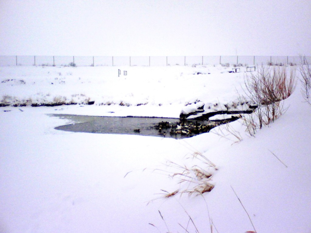
On a snowy Sunday afternoon, we made our way to the “Duck Park” in Rexburg, ID.  When we arrived we found the ducks all gathered around a drainage pipe that had warmed up a portion of the lake enough to melt the ice.  There was limited space, and unfortunately the ducks had to share this cramped space with a dead comrade.  Shown below is the dead comrade, as well as the live ducks.

Shown below I am contemplating giving the dead comrade the kiss of life.

Ducks in Lake Carson Holding Dead Duck

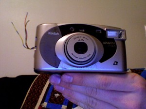
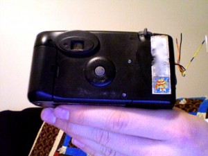
Thor II Camera

ThorIICamera Front ThorIICamera Back ThorIICamera Top

Above are the front, back, and top view of the recovered camera from the  Thor II launch, recovered nearly two years after launch.  This camera differs from that used on the Thor I launch in a number of ways, namely: the film type used was Advantix on ThorII, versus standard 35mm on ThorI. The most significant difference was simply the timing circuit. ThorI used a relatively simply 555 timer circuit, whereas ThorII had a loop running on a microprocessor. Clearly, the 555 method produced good results, as shown on the ThorI page, whereas only 4 relatively poor photographs were recovered from the ThorII camera.

Cheesey Raytracer

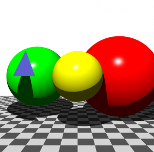
Here’s a Fenisoft 3D raytracer, a sister product with the Fenisoft 3D scanline renderer. The difference here being, of course, that instead of using a scanline approach with a zbuffer, I “project” rays out to determine intersections.

My teacher made the comment that most people show off their raytracers by showing some spheres hovering over a checkerboard. Of course, I have seen this in my days with POV, so I couldn’t resist. Here it is, in all its glory: balls over a checkerboard (with a nice polygon – no meaning implied by using a triangle)

Spheres

Grid Filter

Grid filtering is a useful technique in Artifical Intelligence that lets you determine the true state of your environment from a noisy sensor. As an example, imagine you were a tank in a 3D world that you had never explored. Of course, to make this contrived example less realistic, I will assume you can only “see” what is in the world through your noisy sensor, which basically tells you if there is an object near you. Thing is, by “noisy”, we mean it doesn’t always return accurate data. Instead, most of the time it tells the truth, but because it isn’t perfect it sometimes lies. Using Bayesian reasoning, we can then sample several times in one spot to pin down the true state. Where one single sample might leave us uncertain, more than say 5 or 10 samples should leave us almost certain (but we’re never really 100% sure, just as I feel in my dating life).

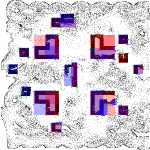
So we implemented this grid filter based of some code that Dr. Goodrich provides. We then produce an occupancy grid where black represents “likely” objects and white represents nothing. We then take it a step further to find corners, and from these corners infer boxes. Below are a few images that show the “believed” state of the world after scanning through it using our sensor and the grid filter logic. On top of this, we have overlaid translucent red or blue squares to indicate obstacles. Youll also notice tick marks around these squares, which are simply to indicate where our corner finding algorithm thought the obstacle edges were.

The cool thing is, this is really simple and useful, since just about any sensor exhibits some noise and hence uncertainty in its interpretation. This particular example works best for static worlds. The Kalman filter is better at modeling dynamic things, seems.

Below: Map of our “world” after using a grid filter and corner detection. Note how “noisy” this is, and yet we were still able to find all our obstacles (the dark black lines). Also note that the colored squares, which are our “believed” obstacles, sometimes cover regions that are larger than what our true obstacle are. For example, around the “L” shaped obstacles, we have a simple square. This works, because we don’t want to get stuck in an “L” anywise (our code for getting our tank out of concave regions isn’t, well, there, really)
Grid Filter

Fenisoft Scanline Renderer

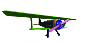
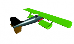
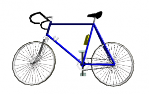
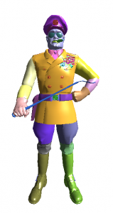
This is one of those projects that seems much cooler to the maker than the observer. Here I have a biplane. What makes it special is that it was rendered using Carson Fenimore’s 3D renderer. If you have never heard of it, that’s ok – that probably won’t change, even after I finalize things with Pixar. It will probably remain anonymous, just as my stock and pay on the deal will be kept secret, leaving me superficially the same, as always, a humble man unwilling to brag.

This renderer was implemented entirely in c++ under Mac OS X and makes use of no external libraries, other than the STL for data containers and OpenGL for drawing 2D points (really 3D points with a Z value of 0). This means this renderer does the following:

  • Polygon rasterization – quads and triangles
  • Z Buffering – using patented hidden secret technology
  • Geometric transformations (scale, translate, rotate)
  • Arbitrary view (camera can be anywhere; specify view angle along with up, look at, and look from vectors
  • Phong shading

The lesson I learned from this is: Don’t be deceived: simple things are often not easy to do. This was not easy to implement – there’s no “cookie-cutter” way to do your own renderer, especially if you have a weak background in linear algebra.

Biplane – in all its magesty
Biplane 2 Biplane 1

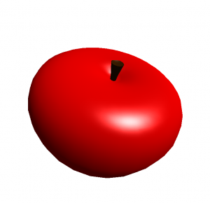
Apple – Notice the Shiny spot thanks to Mr. Phong
Apple

Bike
Bike

General – Very large and complex model
General

The Incredible Hough

A the Hough, now there’s an amazingly simple method for finding circles, lines, and other shapes. Lest this sounds too narrow an application, consider the wild possibility of finding a pool ball. The hough can find these in almost linear time. Amazing!

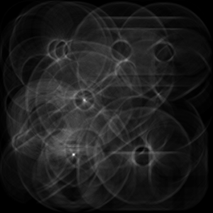
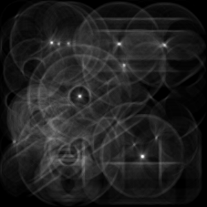
The idea is this: build an “accumulator”, which is really a voting array for parameters describing the object you wish to find. In the case of circles, you could have one accumulator for each approximate radius. Your task is then to go through the source image and find features which “might” be parts of a pool ball; in this case, edges might work. For each point on an edge, we “vote” in a radius around the point. If we do this for all points around a ball, the locus of the ball will have a high number of votes.

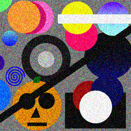
Here’s an example image with some pictures of the accumulator for circles of radius 32 and 48.

Source Image:
Circles

Paramater Space at radius 48
Hough48

Paramater Space at radius 32
Hough32

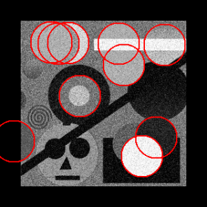
Shown below, is the final result of my Hough Transform for radius 32. Note that it missed one, but had no false positives. Not bad, especially considering I use a general approach that isn’t “hand tuned” to this image.
Huff32Labeled